Running the ISRM Tool on Mac
Last Updated: June 20, 2023
This web page provides a detailed description of how to run the ISRM Tool, built as a collaboration with UC Berkeley, University of Washington, and California’s Office of Environmental Health Hazard Assessment. This document provides a full write-up of how to run this code pipeline on Mac OS. For instructions on how to run the tool in the Google Cloud, please see the instructions here. The Github repository has more information about the code details. Additional details about input file formatting and the control file can be found in the Google Cloud Instruction Document.
Background
The tool is a repository of scripts used for converting emissions to concentrations and health impacts using the InMAP Source Receptor Matrix (ISRM). This first working version of the tool is designed around the California ISRM, however it is possible to run other ISRMs as long as they are in the correct format. For a detailed description of the code repository and to download the code, visit the Github repository here. The following two sections of this page are reproduced from the Github repository.
Purpose and Goals
The Intervention Model for Air Pollution (InMAP) is a powerful first step towards lowering key technical barriers by making simplifying assumptions that allow for streamlined predictions of PM2.5 concentrations resulting from emissions-related policies or interventions.[1] InMAP performance has been validated against observational data and WRF-Chem, and has been used to perform source attribution and exposure disparity analyses.[2, 3] The InMAP Source-Receptor Matrix (ISRM) was developed by running the full InMAP model tens of thousands of times to understand how a unit perturbation of emissions from each grid cell affects concentrations across the grid. However, both InMAP and the ISRM require considerable computational and math proficiency to run and an understanding of various atmospheric science principles to interpret. Furthermore, estimating health impacts requires additional knowledge and calculations beyond InMAP. Thus, a need arises for a standalone and user-friendly process for comparing air quality health disparities associated with various climate change policy scenarios.
The ultimate goal of this repository is to create a pipeline for estimating disparities in health impacts associated with incremental changes in emissions. Annual average PM2.5 concentrations are estimated using the InMAP Source Receptor Matrix for California.
Methodology
The ISRM Health Calculation model works by a series of two modules. First, the model estimates annual average change in PM2.5 concentrations as part of the Concentration Module. Second, the excess mortality resulting from the concentration change is calculated in the Health Module. More details are included in the Github Repository here.
Setting Up on Mac
The tool was developed on MacOS Monterey on the Apple M1 with 16 GB Memory. The instructions below may need to be adapted for different processing capabilities. These instructions assume a base level of comfort navigating your file directories in the terminal. For more information on commands you need for following these instructions, see this article on basic Mac OS commands.
Setting Up Python
Install Python. In order to run the ISRM Tool, the computer must have Python installed. I recommend following the guidance provided by Anaconda for downloading Python on Mac. It is also recommended that you install Anaconda Navigator for ease setting up a virtual environment.
Virtual Environment. The next step is to create a virtual environment for storing the proper versions of libraries required to run this code pipeline. Details on the specific requirements for the ISRM Tool are specified in the Github Repository’s requirements.txt file. To set this up, it is recommended that you download this text file and save it on your computer. There are two ways you can set up your virtual environment.
-
Option 1: Anaconda GUI. Within the Anaconda Navigoator, select the tab “Environments” on the left-hand side. At the bottom, select “Import” to create a new environment from a requirements file. Download the requirements.txt file from the Github repository, and import this file (note: you may need to manually switch your import GUI to search for “Pip requirement files” instead of “Conda environment files”). Set your virtual environment name to “isrm_calcs_env” to be consistent with the rest of this guide. Note: if you are running into Python errors when running the program and you performed your setup this way, you may need to re-try with Option 2 below.
-
Option 2: Terminal. Navigate to your directory of choice using
cd [directory]in your Terminal. Follow the instructions from the official Python documentation here to create your new virtual environment. Set your virtual environment name to “isrm_calcs_env” to be consistent with the rest of this guide. Next, activate that environment by runningsource isrm_calcs_env/bin/activate. Once the environment is created and activated, import the requirements document by runningpython -m pip install -r requirements.txt.
You will test that your virtual environment is set up properly in the next section. If you find that it was not set up properly, you can manually update or install the missing libraries/packages using pip or the Anaconda Navigator GUI.
Clone Repository
It is highly recommended that you clone the repository to keep your code up to date. If you create a static copy, you may miss future changes to the code. You may consider creating a free Github account (instructions) and set up your computer to connect with your account (instructions). However, it is not required to have your own Github account.
Navigate to the Github repository here. To clone the repository:
-
Navigate to the directory where you want the code to be saved from within your Mac Terminal:
cd [path/for/code] -
On the Github interface, click the green “Code” button and copy the https url.
-
In your Terminal, type:
git clone [url]
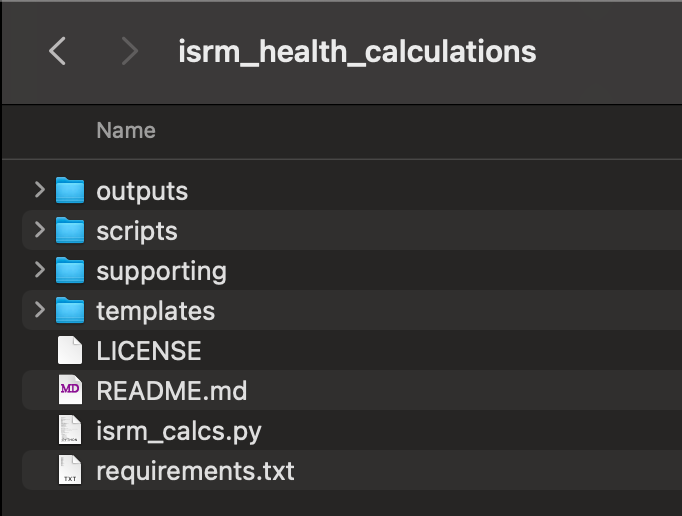
For consistency with this tutorial, name the parent directory “isrm_health_calculations”. Your directory should match the screenshot below.
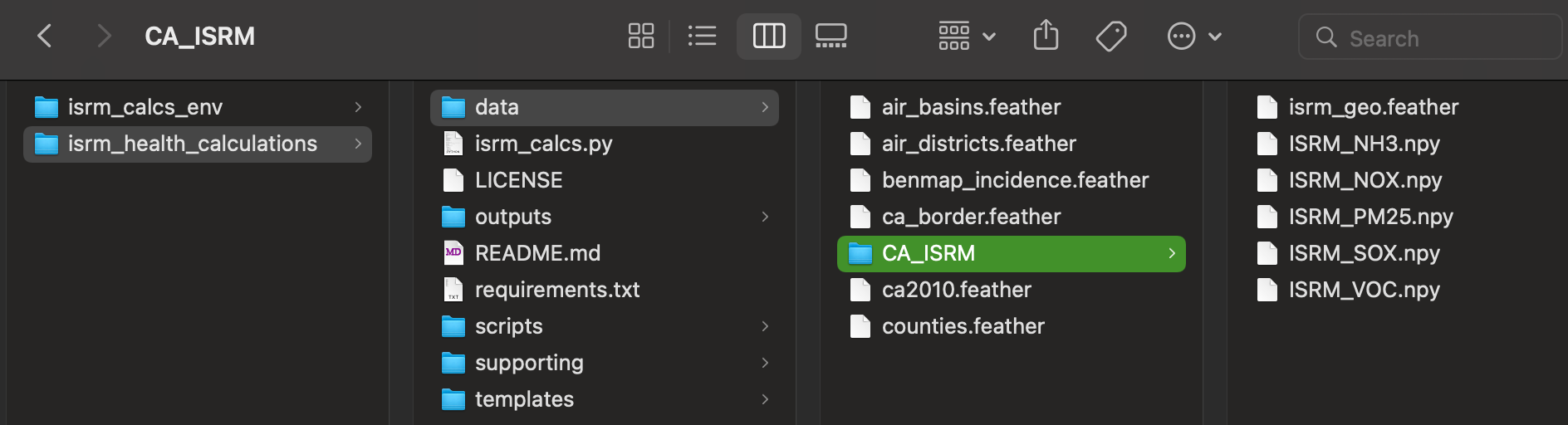
Download Data
Within the isrm_health_calculations folder, create a new folder called “data”. Download the data stored in this Google drive into that folder. Note: you should preserve the structure sub-directory “CA_ISRM” if you intend to use the California ISRM. If you have a different ISRM file, mimic this structure with your ISRM file.
Test Code
Once you have everything ready to go above, your directory should mirror the screenshot below.
Now, you are ready to test the code. We will do this in two steps.
- Confirm Python Works. In the terminal, navigate to the directory where this code is saved. Type the following command, which should return the built-in help statement for the ISRM Tool:
python isrm_calcs.py -h
This is successful if you get the following help message returned (ignore the colors):
usage: isrm_calcs.py [-h] [-i INPUTS]

Runs the ISRM-based tool for estimating PM2.5 concentrations and associated health impacts.

optional arguments:
  -h, --help            show this help message and exit
  -i INPUTS, --inputs INPUTS
                        control file path
- Create a Test File.
Within the “templates” folder of the isrm_health_calculations directory, there should be a text file called “control_file_template.txt”. Copy this file to a directory of choice. For the purposes of this exercise, I will make a copy called “control_file_test.txt”.
Open the text file with a text editor (e.g., TextEdit, Notepad++). Make the following changes. Note - in a future section, I will discuss how to update this control file.
    ╓─────────────────────────────────╖
    ║  HEALTH RUN CONTROLS            ║
    ║  These should be set to Y or N  ║
    ╙─────────────────────────────────╜
    - RUN_HEALTH: N
    - RACE_STRATIFIED_INCIDENCE: N

    ╓────────────────────────────────╖
    ║ RUN CONTROLS                   ║
    ║ These should be set to Y or N  ║
    ╙────────────────────────────────╜
    - CHECK_INPUTS: Y
    - VERBOSE: Y

    ╓──────────────────╖
    ║  OUTPUT OPTIONS  ║
    ╙──────────────────╜
    - REGION_OF_INTEREST:
    - REGION_CATEGORY:
    - OUTPUT_RESOLUTION:
    - OUTPUT_EXPOSURE: N
Back in the terminal in the isrm_health_calcs directory with the isrm_calcs_env virtual environment activated, type the following prompt:
python isrm_calcs.py -i 'path/to/control/file/control_file_test.txt'
If this worked properly, you should get a box pop up with the name of the tool and the version. Then, you should get a number of bulleted messages in simple English about problems running the code. An example is below. These messages are okay and mean that Python is set up properly!
* Issue finding ISRM_NH3.npy in the provided ISRM directory
<< ERROR: Control file was successfully imported but inputs are not correct >>
Running on Mac
The next section will describe how to run ISRM calculations on your Mac provided you have an emissions file. If you want to follow along step-by-step with this guide, feel free to download my sample data. The sample data is the California EMFAC model calendar year 2000 dataset.
Setting Up Emissions File
In order to run the ISRM Tool, you will need to provide it with an emissions input file as either a shapefile, a feather file, or a CSV file (point sources only). Shapefiles can be created using ArcGIS, QGIS, or coding languages like Python or R. Feather files are best created in Python. If you have only point sources, you can import a CSV file using latitude and longitude coordinates from Google Maps (WGS84).
The emissions file needs to have the following columns in order to run properly. Column names are bolded with descriptions following.
- I_CELL: ID column, just needs to be unique
- J_CELL: ID column, just needs to be unique
- Five emissions columns. These can have any units of mass per time, so long as they are all the same.
- PM25
- NH3
- VOC
- NOX
- SOX
- HEIGHT_M: source release height in meters. This can be slightly imprecise, since things are binned into the three layers of the ISRM (0-57 m, 57-140 m, > 760 m)
Save this file in a directory of your choice, but be sure to write this directory down in your notes.
Setting Up Control File
The control file is the central input file for directing your tool run.
- Make a copy of the control file. Within the directory where the tool is saved, find the “templates” folder, and copy the “control_file_template.txt” to a directory of your choice. Note this directory.
- Edit the control file. Open the copy of the control file in a text editor (e.g., TextEdit). A description of each field is below. When finished, save the control file and write the path down in your notes.
| Input | Required? | Description |
|---|---|---|
| Batch Name | No | Provides a name for the batch of runs. |
| Run Name | No | Provides a run-specific name. |
| Emissions Filename | Yes | Provides the path to the emissions file. For shapefiles, use the .shp file. |
| Emissions Units | Yes | Provide the units for emissions (e.g., ton/yr). |
| ISRM Folder | Yes | Provide the path to the folder containing the ISRM files. |
| Population Filename | Yes | Provides the path to the population file. For shapefiles, use the .shp file. |
| Run Health | No | Indicate whether you want health results. If blank, will run only concentrations. |
| Race Stratified Incidence | No | Future option, currently does not do anything. |
| Check Inputs | No | If enabled, will check all of your inputs and then exit. |
| Verbose | No | If enabled, will output more logging statements. |
| Region of Interest | No | If provided an input, will output results only for this region. |
| Region Category | No | If provided an region of input, provide the type of region (e.g., AD = Air District, AB = Air Basin, C = County). |
| Output Resolution | No | If provided, will aggregate results from ISRM grid cell to provided resolution. |
| Output Exposure | No | If enabled, will output population with concentration data. |
| Detailed Conc | No | If enabled, will output concentration data with additional columns for the precursor species. |
## Running the Tool ##
- In the terminal, navigate to the “isrm_health_calculations” directory using
cd [path/to/isrm_health_calculations]. - Before running, make sure that your clone is up to date by running the following command in your terminal:
git pull origin. - Activate the Python virtual environment using:
source isrm_calcs_env/bin/activate - Call the tool by using the following command:
python isrm_calcs.py -i '[path/to/control/file.txt]'. Note that certain computers may be configured to have the Python path variable aspython3instead ofpython. You will know it is working if it starts producing log statements.
Accessing Output Files
The tool will generate outputs each time you run it. All outputs will be uniquely named and saved in the “outputs” folder within the tool directory. The tool will automatically create a sub-directory for all outputs associated with a single run. The batch name and run name (see table above) will be included in the directory with the following structure: out_[batch]_[run]. If the tool detects that an output folder exists with this name, it will increment by one (e.g., out_[batch]_[run]_01, out_[batch]_[run]_02).
Files generated by a run may include:
- A copy of the control file
- A copy of all logging statements printed on the terminal
- Maps of exposure concentrations and/or health incidences (.png files)
- A distribution of exposure by population group percentile
- A sub-directory of shape files (“shapes”) with detailed exposure concentrations and/or health incidences
Having Trouble?
If you have any trouble while working with the tool on your local Mac machine, please let me know! Please send me an email with your issue and I will try to respond as quickly as possible.